神经网络(Neural Network)(下)

• Cost Function
• Backpropagation Algorithm
• Backpropagation Intuition
• Implementation Note: Unrolling Parameters
• Gradient Checking
• Putting it Together
• NN for linear systems
  • Introduction
  • Testing your linear NN
• Reference

Cost Function

Let's first define a few variables that we will need to use: * \(L\) = total number of layers in the network * \(s_l\)= number of units (not counting bias unit) in layer \(l\) * \(K\) = number of output units/classes

Recall that in neural networks, we may have many output nodes. We denote \(h_Θ(x)_k\) as being a hypothesis that results in the \(k^{th}\) output.

Our cost function for neural networks is going to be a generalization of the one we used for logistic regression.

Recall that the cost function for regularized logistic regression was:

\[J(θ)=−\frac{1}{m}[∑^m_{i=1}y^{(i)}log(h_θ(x^{(i)}))+(1−y^{(i)})log(1−h_θ(x^{(i)}))]+\frac{λ}{2m}∑^n_{j=1}θ^2_j\]

For neural networks, it is going to be slightly more complicated:

\(J(Θ)=−\frac{1}{m}[∑^m_{i=1}∑_{k=1}^Ky^{(i)}_klog((h_Θ(x^{(i)}))_k)+(1−y^{(i)}_k)log(1−(h_Θ(x^{(i)}))_k)]+\frac{λ}{2m}\sum_{l=1}^{L−1}\sum_{i=1}^{s_l}\sum_{j=1}^{s_l+1}(Θ^{(l)}_{j,i})^2\)

Alt text

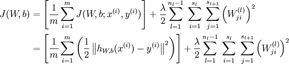
We have added a few nested summations to account for our multiple output nodes. In the first part of the equation, between the square brackets, we have an additional nested summation that loops through the number of output nodes.

In the regularization part, after the square brackets, we must account for multiple theta matrices. The number of columns in our current theta matrix is equal to the number of nodes in our current layer (including the bias unit). The number of rows in our current theta matrix is equal to the number of nodes in the next layer (excluding the bias unit). As before with logistic regression, we square every term.

Note: * the double sum simply adds up the logistic regression costs calculated for each cell in the output layer; * the triple sum simply adds up the squares of all the individual Θs in the entire network. * the i in the triple sum does not refer to training example i

Backpropagation Algorithm

"Backpropagation" is neural-network terminology(术语) for minimizing our cost function, just like what we were doing with gradient descent in logistic and linear regression.

Our goal is to compute: \[min_ΘJ(Θ)\]

That is, we want to minimize our cost function \(J\) using an optimal set of parameters in theta.

In this section we'll look at the equations we use to compute the partial derivative of \(J(Θ)\): \[\frac{∂}{∂Θ^{(l)}_{i,j}}J(Θ)\]

In backpropagation we're going to compute for every node: \(δ^{(l)}_j\) = "error" of node \(j\) in layer \(l\)

Recall that \(a^{(l)}_j\) is activation node \(j\) in layer \(l\).

For the last layer, we can compute the vector of delta values with: \[δ^{(L)}=a^{(L)}−y\]

Alt text

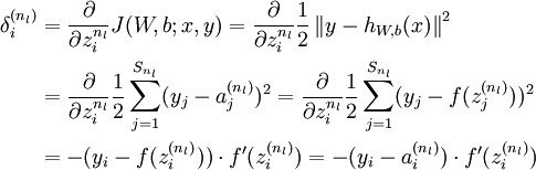
Where \(L\) is our total number of layers and \(a^{(L)}\) is the vector of activation units for the last layer. So our "error values" for the last layer are simply the differences of our actual results in the last layer and the correct outputs in \(y\).

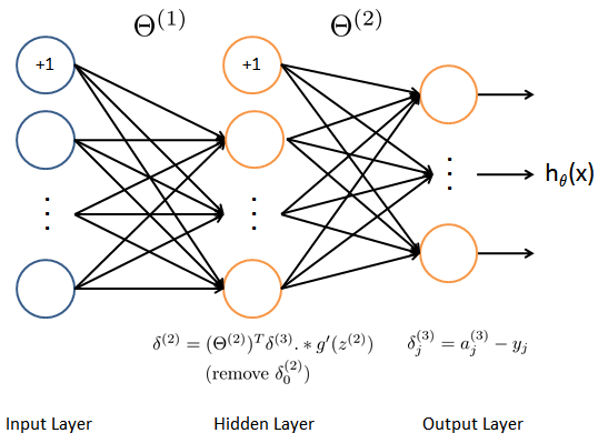
To get the delta values of the layers before the last layer, we can use an equation that steps us back from right to left: \[δ^{(l)}=((Θ^{(l)})^Tδ^{(l+1)}) .∗ g′(z^{(l)})\]

Alt text

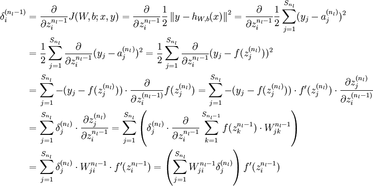
The delta values of layer \(l\) are calculated by multiplying the delta values in the next layer with the theta matrix of layer \(l\). We then element-wise multiply that with a function called \(g'\), or g-prime, which is the derivative of the activation function \(g\) evaluated with the input values given by \(z^{(l)}\).

The g-prime derivative terms can also be written out as: \[g′(z^{(l)})=a^{(l)} .∗ (1−a^{(l)})\]

This can be shown and proved in calculus.

\[g(z)=\frac{1}{1+e^{−z}}\] \[\begin{array}{lcr} \frac{∂g(z)}{∂z}=−(\frac{1}{1+e^{−z}})^2\frac{∂}{∂z}(1+e^{−z}) \\ \ \ \ \ \ \ \ \ \ =−(\frac{1}{1+e^{−z}})^2e^{−z}(−1) \\ \ \ \ \ \ \ \ \ \ =(\frac{1}{1+e^{−z}})(\frac{1}{1+e^{−z}})(e^{−z}) \\ \ \ \ \ \ \ \ \ \ =(\frac{1}{1+e^{−z}})(\frac{e^{−z}}{1+e^{−z}}) \\ \ \ \ \ \ \ \ \ \ =g(z)(1−g(z)) \end{array}\]

The full backpropagation equation for the inner nodes is then: \[δ^{(l)}=((Θ^{(l)})^Tδ^{(l+1)}) .∗ a^{(l)} .∗ (1−a^{(l)})\]

We can compute our partial derivative terms by multiplying our activation values and our error values for each training example t: \[\frac{∂J(Θ)}{∂Θ^{(l)}_{i,j}}=\frac{1}{m}\sum^m_{t=1}a^{(t)(l)}_jδ^{(t)(l+1)}_i\]

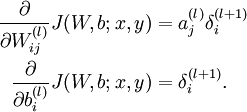\[\frac{\partial}{\partial W^{(l)}_{ij}} J(W,b;x,y)= \frac{\partial}{\partial z^{(l+1)}_{i}}J(W,b;x,y) \cdot \frac{\partial z^{(l+1)}_i}{\partial W^{(l)}_{ij}} = a^{(l)}_j\delta^{(l+1)}_i\]

This however ignores regularization, which we'll deal with later.

Note: \(δ^{l+1}\) and \(a^{l+1}\) are vectors with \(s_{l+1}\) elements. Similarly, \(a^{(l)}\) is a vector with \(s_l\) elements. Multiplying them produces a matrix that is \(s_{l+1}\) by \(s_l\) which is the same dimension as \(Θ^{(l)}\). That is, the process produces a gradient term for every element in \(Θ^{(l)}\). (Actually, \(Θ^{(l)}\) has \(s_{l+1} + 1\) rows, so the dimensionality is not exactly the same).

We can now take all these equations and put them together into a backpropagation algorithm:

Backpropagation Algorithm

Backpropagation Algorithm

• Given training set {(\(x^{(1)}\), \(y^{(1)}\))⋯(\(x^{(m)}\), \(y^{(m)}\))}
• Set \(Δ^{(l)}_{i,j} := 0\) for all (\(l\), \(i\), \(j\))
• For training example \(t=1\) to \(m\):
  • Set \(a^{(1)} := x^{(t)}\)
  • Perform forward propagation to compute \(a^{(l)}\) for \(l=2,3,…,L\)
  • Using \(y^{(t)}\), compute \(δ^{(L)}=a^{(L)}−y^{(t)}\)
  • Compute \(δ^{(L−1)}\),\(δ^{(L−2)}\),…,\(δ^{(2)}\) using \(δ^{(l)}=((Θ^{(l)})^Tδ^{(l+1)}) .∗ a^{(l)} .∗ (1−a^{(l)})\)
  • \(Δ^{(l)}_{i,j} :=Δ^{(l)}_{i,j}+a^{(l)}_jδ^{(l+1)}_i\) or with vectorization, \(Δ^{(l)} :=Δ^{(l)}+δ^{(l+1)}(a^{(l)})^T\)
• \(D^{(l)}_{i,j} := \frac{1}{m}(Δ^{(l)}_{i,j}+λΘ^{(l)}_{i,j})\) If \(j≠0\)
• \(D^{(l)}_{i,j} := \frac{1}{m}Δ^{(l)}_{i,j}\) If \(j=0\)

The capital-delta matrix is used as an "accumulator" to add up our values as we go along and eventually compute our partial derivative.

The actual proof is quite involved, but, the \(D^{(l)}_{i,j}\) terms are the partial derivatives and the results we are looking for: \(D^{(l)}_{i,j} = \frac{∂J(Θ)}{∂Θ^{(l)}_{i,j}}\).

Backpropagation Intuition

The cost function is: \(J(Θ)=−\frac{1}{m}[∑^m_{i=1}∑_{k=1}^Ky^{(i)}_klog((h_Θ(x^{(i)}))_k)+(1−y^{(i)}_k)log(1−(h_Θ(x^{(i)}))_k)]+\frac{λ}{2m}\sum_{l=1}^{L−1}\sum_{i=1}^{s_l}\sum_{j=1}^{s_l+1}(Θ^{(l)}_{j,i})^2\)

If we consider simple non-multiclass classification (k = 1) and disregard regularization, the cost is computed with: \[cost(t)=y^{(t)}log(h_θ(x^{(t)}))+(1−y^{(t)})log(1−h_θ(x^{(t)}))\]

More intuitively you can think of that equation roughly as: \[cost(t)≈(h_θ(x^{(t)})−y^{(t)})^2\]

Intuitively, \(δ^{(l)}_j\) is the "error" for \(a^{(l)}_j\) (unit \(j\) in layer \(l\))

More formally, the delta values are actually the derivative of the cost function: \[δ^{(l)}_j=\frac{∂}{∂z^{(l)}_j}cost(t)\]

Recall that our derivative is the slope of a line tangent to the cost function, so the steeper the slope the more incorrect we are.

Note: In lecture, sometimes i is used to index a training example. Sometimes it is used to index a unit in a layer. In the Back Propagation Algorithm described here, t is used to index a training example rather than overloading the use of i.

Implementation Note: Unrolling Parameters

With neural networks, we are working with sets of matrices: \(Θ_1\), \(Θ_2\), \(Θ_3\),… \(D_1\), \(D_2\), \(D_2\),…

In order to use optimizing functions such as "fminunc()", we will want to "unroll" all the elements and put them into one long vector:

thetaVector = [ Theta1(:); Theta2(:); Theta3(:); ]
deltaVector = [ D1(:); D2(:); D3(:) ]

If the dimensions of Theta1 is 10x11, Theta2 is 10x11 and Theta3 is 1x11, then we can get back our original matrices from the "unrolled" versions as follows:

Theta1 = reshape(thetaVector(1:110),10,11)
Theta2 = reshape(thetaVector(111:220),10,11)
Theta3 = reshape(thetaVector(221:231),1,11)

Gradient Checking

Gradient checking will assure that our backpropagation works as intended. We can approximate the derivative of our cost function with: \[\frac{∂}{∂Θ}J(Θ) ≈ \frac{J(Θ+ϵ)−J(Θ−ϵ)}{2ϵ}\]

With multiple theta matrices, we can approximate the derivative with respect to \(Θ_j\) as follows: \[\frac{∂}{∂Θ_j}J(Θ) ≈ \frac{J(Θ_1,…,Θ_{j+ϵ},…,Θ_n)−J(Θ_1,…,Θ_{j−ϵ},…,Θ_n)}{2ϵ}\]

A good small value for \(ϵ\) (epsilon), guarantees the math above to become true. If the value be much smaller, may we will end up with numerical problems. The professor Andrew usually uses the value \(ϵ=10^{−4}\).

We are only adding or subtracting epsilon to the \(Θ_j\) matrix. In octave we can do it as follows:

epsilon = 1e-4;
for i = 1:n,
  thetaPlus = theta;
  thetaPlus(i) += epsilon;
  thetaMinus = theta;
  thetaMinus(i) -= epsilon;
  gradApprox(i) = (J(thetaPlus) - J(thetaMinus))/(2*epsilon)
end;

We then want to check that gradApprox ≈ deltaVector.

Once you've verified once that your backpropagation algorithm is correct, then you don't need to compute gradApprox again. The code to compute gradApprox is very slow.

Putting it Together

First, pick a network architecture; choose the layout of your neural network, including how many hidden units in each layer and how many layers total. * Number of input units = dimension of features \(x^{(i)}\) * Number of output units = number of classes * Number of hidden units per layer = usually more the better (must balance with cost of computation as it increases with more hidden units) * Defaults: 1 hidden layer. If more than 1 hidden layer, then the same number of units in every hidden layer.

Training a Neural Network

1. Randomly initialize the weights
2. Implement forward propagation to get \(h_θ(x^{(i)})\)
3. Implement the cost function
4. Implement backpropagation to compute partial derivatives
5. Use gradient checking to confirm that your backpropagation works. Then disable gradient checking.
6. Use gradient descent or a built-in optimization function to minimize the cost function with the weights in theta.

When we perform forward and back propagation, we loop on every training example:

for i = 1:m,
   Perform forward propagation and backpropagation using example (x(i),y(i))
   (Get activations a(l) and delta terms d(l) for l = 2,...,L

NN for linear systems

Introduction

The NN we created for classification can easily be modified to have a linear output.

First solve the 4th programming exercise. You can create a new function script, nnCostFunctionLinear.m, with the following characteristics * There is only one output node, so you do not need the 'num_labels' parameter. * Since there is one linear output, you do not need to convert y into a logical matrix. * You still need a non-linear function in the hidden layer. * The non-linear function is often the tanh() function - it has an output range from -1 to +1, and its gradient is easily implemented. Let \(g(z)=tanh(z)\). * The gradient of tanh is \(g′(z)=1−g(z)^2\). Use this in backpropagation in place of the sigmoid gradient. * Use linear regression for the NN output (do not use a sigmoid function on the output layer). * Cost computation: Use the linear cost function for \(J\) (from ex1 and ex5) for the unregularized portion. For the regularized portion, use the same method as ex4. * Where reshape() is used to form the Theta matrices, replace 'num_labels' with '1'.

You will also need to create a predictLinear() function, using the tanh() function in the hidden layer, and a linear output.

Testing your linear NN

Here is a test case for your nnCostFunctionLinear()

% inputs
nn_params = [31 16 15 -29 -13 -8 -7 13 54 -17 -11 -9 16]'/ 10;
il = 1;
hl = 4;
X = [1 ; 2 ; 3];
y = [1 ; 4 ; 9];
lambda = 0.01;

% command
[j g] = nnCostFunctionLinear(nn_params, il, hl, X, y, lambda)

% results
j =  0.020815
g =
    -0.0131002
    -0.0110085
    -0.0070569
     0.0189212
    -0.0189639
    -0.0192539
    -0.0102291
     0.0344732
     0.0024947
     0.0080624
     0.0021964
     0.0031675
    -0.0064244

Now create a script that uses the 'ex5data1.mat' from ex5, but without creating the polynomial terms. With 8 units in the hidden layer and MaxIter set to 200, you should be able to get a final cost value of 0.3 to 0.4. The results will vary a bit due to the random Theta initialization. If you plot the training set and the predicted values for the training set (using your predictLinear() function), you should have a good match.

Reference

• 机器学习 Andrew Ng
• UFLDL教程